Freezing the Panes
Occasionally a worksheet is so large, you cannot view the column or row headings and all the data at the same time. When this happens, it is difficult to view the headings for the data in the worksheet. For example, in a worksheet containing sales figures for several hundred sales representatives, you cannot view the column headings and the representatives at the bottom of the list at the same time. To solve this problem, you can freeze worksheet titles in panes. Freezing panes prevents the row and column headings from scrolling out of view as you navigate the worksheet. Frozen panes are indicated by a line above a row and a line to the left of a column.

|
|
|
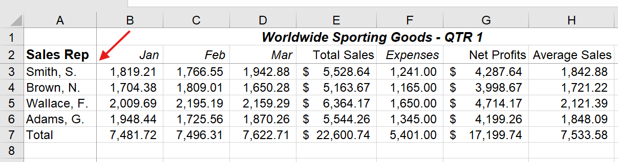
1. To freeze both row and column headings, place the cursor in the cell directly below the column headings you want to freeze and to the right of the row headings you want to freeze.
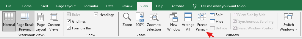
2. Select the View tab.
3. Select the Freeze Panes button in the Window group.
4. Select Freeze Panes.
The rows above and the columns to the left of the active cell are frozen. See the intersection of B3. Once cell is frozen, you can then easily enter data to the far right without having to scroll for each line of data.
|
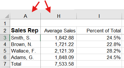
Once the intersecting cell is frozen and you scroll to the right, you’ll see columns A and H are right next to each other in the screenshot below — no tabbing to the many columns to the right to perform data entry!
Unfreezing the Panes
After you have frozen headings in a large worksheet, you can unfreeze the panes. Unfreezing removes the panes so that title rows or columns are no longer frozen on the screen.
1. Select the View tab.
2. Select the Freeze Panes button in the Window group.
3. Select the Unfreeze Panes command.
The headings are no longer frozen.